Flow Injection Fluidics


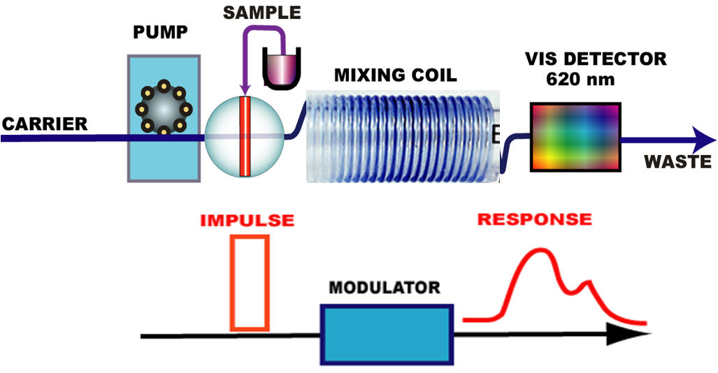
Upon acceleration the injected zone disperses within the carrier stream, forming a parabolic profile (0.3.6). The thus formed concentration gradient expands axially as it passes through a mixing coil. This process is visualized here by injecting a blue dye, which is shown to form a typical concentration gradient, as it flows through a coiled tube. A colorimetric monitoring of this concentration gradient yields a response curve, which is the result of axial and radial dispersion of the initial square impulse. Note that this Residence Time Distribution curve (RTD) does not provide information on underlying mechanism of the dispersion processes, since it depicts the flow system as a black box. Note that the tracer dye method is applicable not only to cFI but also to pFI and SI, since all these techniques share the same underlying fluidic principles. Consequently the principal parameters such as S1/2, t etc. derived from RTD, are suitable for optimization of the dispersion process for all flow injection techniques (Chapter 0).
1.2.1.